Casual videos shot with a smartphone can often suffer from shakiness. Software-based video stabilization methods have been actively developing over the last years and can make such videos look much more professional and fluid. We have just released Deshake, our video stabilizer app for iOS that can enable faster than real-time video processing. In this article, we are going to overview the video stabilization techniques available and discuss some of engineering challenges we have faced during the development.
Video Stabilization
Generally speaking, every video stabilization algorithm has to implement two steps:
- Analyse motion between the consecutive frames of the video. The sequence of such motions will constitute a trajectory which is usually a pretty shaky one.
- Build a smoothed version of the trajectory and attempt to re-create the video as if it were shot along this new trajectory.
The biggest problem here is that algorithm mostly has to operate with frames only. Those are 2D images which are tremendously simplified representations of the real dynamic 3D world. A lot could have happened in that world between two adjacent frames. Even if we ignore the movements of the objects shot, the camera alone can change its location, orientation or even some internal parameters like focal length or zoom level.
To demonstrate why the problem is so arduous, let us ignore everything but the camera movement for a moment. There are 6 degrees of freedom in the movement already — 3 for location (x, y and z) and 3 for orientation (yaw, roll, pitch). Do we have any chance to reconstruct them at least? Well, in a sense we cannot. It is well-known that based on only two 2D images of a static 3D world taken with the same camera (no focal length modifications, etc.) you can’t positively determine the relative movement of such camera between the shots. To determine the movement you have to know some external data: it may be the camera parameters (that’s why in 3D scanning and other applications calibrated cameras are widely used) or some insights on the scene shot (for instance, if you have shot a building you can solve the problem based on the assumption that its windows are rectangular and walls are perpendicular to the ground).
Back to our case. We have much more than just two images and for a certain point of view motion estimation does not necessarily require camera position estimation. At this point, different stabilization algorithms diverge a lot.
The most complicated and reckless algorithms attempt to reconstruct the full 3D picture based on the frames only. As we already know, even in a perfectly static world you cannot do this with two adjacent frames: any reconstruction would necessarily include camera movement estimation which is impossible as you know. However, three frames would be sufficient (google up trifocal tensor, multi view 3D reconstruction and so on). But in practice to accommodate dynamism of the scene and types of instability, such algorithms have to account multiple consecutive frames, calibrate camera on the fly and do some other non-trivial stuff. It is still quite unstable; for example, one known weakness of such algorithms is camera rotations without movement. In such a case there is almost no effect of parallax (i.e., relative shifting of objects positioned at different distances from the camera) in the image and 3D reconstruction techniques may simply fail. It is also extremely slow: probably the most notorious attempt in the field is Microsoft’s First-Person Hyperlapse which spends minutes (!) on a single video frame. Certainly there are some benefits in such an approach: by knowing real 3D positions of the camera you can easily draw a smooth physically correct alternative path in all 6 degrees of freedom. Then, with a reconstructed 3D scenery you can literally render the stabilized video as if it were really shot with a camera moving along that path.
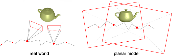
The most conventional models pretend that the world is two-dimensional. For them the camera is just a rectangular framework moving over an infinite plane. This may appear a highly simplistic approach, but in real life for each pair of adjacent frames this simplification often works pretty well. From the mathematical point of view we can call it the similarity motion model. With few degrees of freedom (4 with scaling, otherwise 3) and very easy transform rules, it has proven itself robust and computationally efficient. Moreover, you can physically interpret the trajectory you get from this model: the camera is moving along a polyline on a plane, rotating here and there. Such an interpretation, although it is not exactly reflecting the real world situation, is a real helper at the smoothing step: it can even imitate camera motions used by professional cameramen (see article Auto-Directed Video Stabilization with Robust L1 Optimal Camera Paths to learn more).
In fact, you don’t have to use this very planar model: there are other classes of motions to choose from. For example, you can assume the world to be a sphere with a camera in its center which can rotate between frames. Such a rotational model is also often used in panorama stitching. This model can simulate some non-trivial perspective transforms between frames that are out of scope for the similarity model.
So the overall idea is to leave frames in 2D, treating a single frame as a solid piece of plane that can be moved around, scaled or even skewed, but still remains a solid piece. The benefits of this approach are high computational speed and robustness. The downside is that it is restricted to the allowed transforms.
There are also some intermediate solutions we can call 2.5D. The general idea is that we track points as they move between frames, choose long enough and consistent tracks and consider them, without any attempt to interpret what is happening either in 3D or on the frames, as the motions of interest. Then we smooth such tracks and try to bend each frame so that the points move from their original positions to the smoothed tracks. The trick here is that we use, both during smoothing and bending, the underlying ideas of true 3D reconstruction (e.g., epipolar geometry), but without any actual 3D reconstruction. From the performance viewpoint such algorithms are also somewhere between 2D and 3D.
Our main goal was to achieve at least real-time video processing on modern smartphones, so for us there were no options but to stick to 2D. As for the motion model, we use neither the similarity model nor rotational model, but some experimental model of our own.
Motion Between Frames
As we have chosen how to stabilize motions, the question now is how to determine the motions to be stabilized. The obvious way to go is to analyze frames. But how exactly should this be done?
What we need here is called, in computer vision, Image Registration. Those are techniques which align several images of the same scene. Generally speaking, such techniques can be classified into the spatial domain methods and frequency domain methods. Spatial methods compare pixel colours, while frequency methods first use some tricky algorithms like Fast Fourier Transform to transform the array of pixels into a set of waveforms and then look for correlations between them. The spatial methods in turn can be classified into intensity-based and feature-based methods. The intensity-based methods deal with intensity patterns of the whole image while feature-based methods try to find correspondences between some local features such as points, lines or contours. The feature-based methods are most widely used for video stabilization today: they are faster as they don’t have to deal with the whole images most of the time and they are more precise, as single features can be aligned very accurately, sometimes up to subpixels.
There are some implementation variations of feature-based image registration, but let’s focus on the approach that we have adopted. First of all, we use points as features. We select a set of points on a frame and then try to determine what locations those points are moved to on the next frame. Such movement of single points on a frame is called the optical flow. The optical flow estimation is based on the assumptions that:
- patches of pixels around a point and its correspondence in the next frame are almost identical and
- the point has probably not moved too far between two adjacent frames.
So we compare the patches of pixels around the point with those not far from it on the next frame and choose the one with the greatest resemblance. To do it efficiently, we use the pyramidal variation of Lucas-Kanade method.
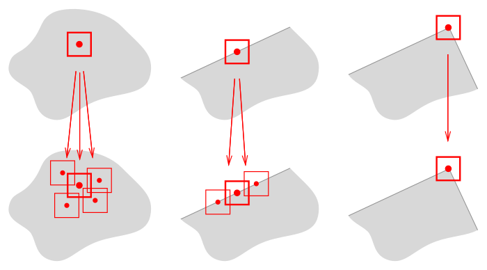
There is still one important issue to solve, i.e., which set of points to choose as features? It turns out that the best candidates for features are corners (i.e. vertices of angles) on the image. The rationale is as follows: all points can be tentatively classified into internal points, border points and corner points. If you choose an internal point as a feature, not only a patch around the true image of that point on the next frame will be similar to the original patch, but almost any of its neighbours will suffice. For a border point, all of the true image neighbours along the border will have confusingly similar patches in the next frame. But the corners are not affected by such a problem. Interestingly enough, the fact that only corners are good to determine the motion is not a deficiency of the particular algorithm we are using, in absence of corners even the human brain can misidentify motions. This problem is known in motion perception as the Aperture Problem.
So we need to find corners in the image. For this we use a variation of Harris Corner Detector.
After we have selected the features on the image and found their correspondences on the next frame, we have to deduce the motion between frames (i.e., the transform). This step depends on the motion model chosen, but generally you just optimize your model iteratively or in some other way to minimize the error between your model’s prediction and real point movement just estimated.
That was the obvious way: you have frames, you analyze them. But there is an alternative way also. What if you have some external sensor and its data is recorded alongside the video? Certain attempts have already been done in this area. An apparent choice for such a sensor is the accelerometer (and/or gyroscope) of a device. Most modern smartphones already have it; it can provide surprisingly precise data at a high rate (higher than the video frame rate) and it literally gives you the raw motion between frames. There are solutions based on this approach, most notably Instagram’s Hyperlapse. Pros are apparent: the biggest problem here is to calibrate the accelerometer/gyroscope correctly (its timeline can differ a little from the camera’s timeline, and it can have some drift). After that you get the required data almost for free (from the computational point of view). The downside is that the only data you have is the rotational component of the motion and you can say nothing of the translational shaking or other types or movement like in shooting the moving target: for instance, in shooting videos from a running car). Another clear downside is that the video should be shot from a given app. So if you have shot it previously or want to shoot it with another app to use some filters or exposure/focus controls, you just won’t be able to stabilize the video.
Another curious example of using external sensors for motion estimation is the recent attempts to use a depth camera (e.g. Kinect) alongside with a normal camera. That way you have a 3D scene without the need to reconstruct it, which gives you the pros of a fully 3D approach without most of its cons. The problem is that the depth camera is not good at big distances (i.e., it is not applicable to outdoor shooting yet). Other issues include calibration and alignment of the colour camera with the depth camera. And, yes, the depth cameras are not sufficiently widespread yet.
OpenCV
As its name suggests, OpenCV is an open-source computer vision library. It contains highly optimized implementations for many computer vision algorithms (including some accelerated versions for CUDA, NEON, etc.). It is cross-platform (written in C++) and has become a de-facto industry standard. Unsurprisingly, OpenCV already contains a video stabilization implementation, accidentally it is exactly the one we have just described. But an attempt to run this implementation as it is has not been quite cheerful.
As a test case we have selected a 1-minute full HD video captured with an iPhone at 30 frames per second. OpenCV’s native implementation has spent 13 minutes to process this video, and a typical user won’t wait for so long. So we aimed at speeding-up the processing 13-fold. Before discussing our results, let’s review some details specific to the current OpenCV implementation.
First of all, OpenCV on iPhone runs totally on CPU. At the moment, OpenCV supports only CUDA-based GPU computing, and it is not available on iPhone. Moreover, the OpenCV implementation has been designed to be cross-platform, and although some parts of the algorithm are optimized for specific platforms (for example, video file decoding on iPhone uses Apple’s optimized AVFoundation framework), the general pipeline had to remain suboptimal.
To be more specific, OpenCV stores single frames most of the time as RGB encoded images (as it requires them either way to output stabilized frames), but the computer vision algorithms (including feature detection, optical flow estimation, etc.) require grayscale images as their input. That’s why OpenCV converts RGB frames to grayscale each time it needs to pass them to individual steps: hence it performs the grayscale conversion several times for each input frame. Another example: besides the frame, the optical flow algorithm needs a series of auxiliary images constituting what is called a Gaussian pyramid; this pyramid is also computed more than once for each frame.
So the first step for us was to remove such and similar redundancies from the computations.
Our Solution
As I have already mentioned, OpenCV does grayscale conversion multiple times for each frame. Yet the problem is deeper. In fact, during motion estimation (which is run as a single-pass pre-processing through a video file) there is no single algorithm in the pipeline that requires an RGB-encoded frame. But you may be surprised to know that frames in video files are usually stored using the YUV colour space invented to transmit the colour television signal via the black-and-white infrastructure. Its Y component represents luma (i.e. brightness) of the pixel and U, V are responsible for chrominance (colour itself). Therefore, the problem is that OpenCV first has to convert from grayscale (Y component) to RGB using additional information (UV components) and then to convert it multiple times back to grayscale. To eliminate it, but still maintain fast video decoding on iOS, you can use AVFoundation in combination with Core Video’s pixel buffers. Intentionally simplified setup code for asset reading with proper preparations may look like this:
[gist id=d2a4fe1eb3ab723a2b56122ae05414b9]
Here the kCVPixelBufferPixelFormatTypeKey key tells AVFoundation to provide for each frame a Core Video buffer and the format kCVPixelFormatType_420YpCbCr8Planar is chosen to eliminate any unneeded colour conversions during decoding. Note also that AVFoundation sets the alwaysCopiesSampleData property of videoOutput to YES by default. It means that each frame’s data is copied after decoding, which is not required in our case. So setting this property to NO can sometimes give you a performance boost. The colour format used here is planar, for us it means that the Y component will be stored in a continuous region of memory separately from others, which makes processing we have to do both simpler and faster.
Single frame reading can look like this:
[gist id=a6141d20959466787f497943ac5493d0]
It’s important to use CVPixelBufferGetBaseAddressOfPlane here instead of the standard CVPixelBufferGetBaseAddress as the colour format is planar. If you are not familiar with the Core Video framework, please note that in this example you can only process pixels pointed by grayscalePixels before CVPixelBufferUnlockBaseAddress is called, and you are not allowed to modify them (as the read-only access here was requested).
After we have removed all the unnecessary colour conversions and other computations and did some other memory optimizations, the processing speed still remained far from desired. So the next decision was to downscale frames before processing. That may sound unreasonable, but the reality is that the full frame definition gives you more noise than data for stabilization. We have downscaled frames to half of their original size easily using cv::resize. It is the OpenCV function already highly optimised, including even NEON support on iOS.
And that was still not enough. The next heuristic we have applied is as follows. Feature detection is quite a computationally intensive algorithm; in fact, more than 60% of time at that moment was consumed by this step. But as we have estimated the optical flow, we have already computed frame-to-frame feature mapping. So, if on the previous frame the points were good enough to be considered features (they had high ‘cornerness’), than probably after mapping they will still remain good. Why not just reuse this knowledge? So, we can compute features on a given frame and then do not recompute them from scratch for a few next frames: each time we can use the points we get after optical flow estimation as features. So we have keyframes, i.e., those for which we run the real feature detector, and all the other frames get their set of features for free, as we compute the optical flow either way.
After all these optimizations, the processing time of a 1-minute video has decreased from 13 minutes to 42 seconds. Well, that is already faster than real-time but still not fast enough for us. In fact, all this time we consciously left one optimization in reserve, that is, parallelization. As you certainly know, all modern iOS devices have 2-core CPUs, and this can potentially double your computational power at least if you know how to use them efficiently. In fact, OpenCV already uses some parallelization features, but for video stabilization the support is not extensive enough.
Video stabilization has turned out to be an interesting problem in context of parallelization. You can see that, for each frame we may want at some point to: read it (that is, to request the next decoded frame from AVAsset reader), downscale it, construct the Gaussian pyramid for it, find features on it (if it is a keyframe), compute the optical flow (between it and the next one) — that’s 5 potential operations for a single frame. The problem is not the count, but the interdependencies between them, which you can see on the scheme:
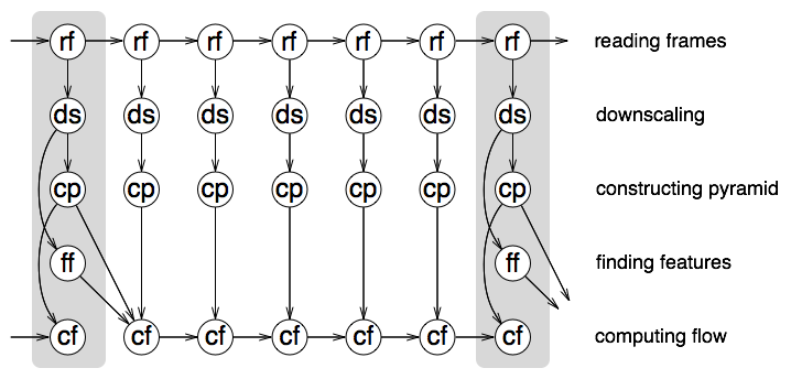
The scheme shows the operations for a single frame in columns, while the keyframes are marked with the darker background. The arrows connect an operation with the dependent operations. In fact, the distance between keyframes in our case is 8 rather than 6, but the general idea is the same. So, we have lots of operations to do and we have to manage dependencies between them somehow: NSOperationQueue is a perfect fit for the task. We apply a standard scheme: one serial operation queue is used to coordinate the process (i.e., dispatch new operations for the individual frames) and respond to requests from the user (i.e., begin processing, cancel processing, etc.) and another concurrent operation queue is used for all the frame operations. This works great. The only potential issue here is, as the video is processed a tail of processed dependencies is piled up: on the scheme you can see that each compute optical flow operation has most of the previous operations as its dependency in some generation. Such operations remain in memory and can potentially mess some of your plans. However, you can easily remove them if you apply the following code to already processed operations (for example, it is sufficient to apply it to the keyframe read and flow operations):
[gist id=2ffeaa9c81ab9d7d9858b1fcbca589c9]
This solution gives us an almost perfect parallelization: debug shows ~90% of the CPU resources is consumed by our processing code and the other ~10% is used by the system, probably for video decoding.
So after all these optimizations including parallelization, our test with a 1-minute full HD video processing takes 22 seconds only.